Between Method Type Comparisons¶

This notebook compares across different methods, running them on the same set of simulations, and comparing the results.

Time Domain methods that are compared:

Autocorrelation decay rate
Hurst exponent
Detrended Fluctuation Analysis
Higuchi Fractal Dimension
Hjorth Complexity
Lempel Ziv Complexity
Sample Entropy
Permutation Entropy

In addition, the above methods are compared to frequency domain methods:

Spectral Parameterization

# Setup notebook state
from nbutils import setup_notebook; setup_notebook()

import numpy as np
import matplotlib.pyplot as plt

from neurodsp.sim import sim_combined
from neurodsp.plts.utils import make_axes
from neurodsp.utils import set_random_seed

# Import custom project code
from apm.io import APMDB
from apm.run import run_comparisons
from apm.analysis import compute_all_corrs, compute_corrs_to_feature, unpack_corrs
from apm.plts import plot_dots, plot_corr_matrix
from apm.plts.multi import plot_results_rows, plot_results_all
from apm.plts.settings import LABELS, COLORS
from apm.plts.utils import figsaver
from apm.methods import (autocorr_decay_time, hurst, dfa, higuchi_fd, hjorth_complexity,
                         lempelziv, sample_entropy, perm_entropy, specparam)
from apm.methods.settings import (AC_DECAY_PARAMS, HURST_PARAMS, DFA_PARAMS, HFD_PARAMS,
                                  HJC_PARAMS, LZ_PARAMS, SA_ENT_PARAMS, PE_ENT_PARAMS)
from apm.sim.defs import SIM_SAMPLERS
from apm.utils import print_all_corrs

Settings¶

# Define settings
f_range = [1, 50]
specparam_kwargs = {'min_peak_height' : 0.05, 'fs' : SIM_SAMPLERS.fs, 'f_range' : f_range}

# Settings for running comparisons
RETURN_PARAMS = True

# Settings for saving figures
SAVE_FIG = True
FIGPATH = APMDB().figs_path / '42_between_comp'

# Create helper function to manage figsaver settings
fsaver = figsaver(SAVE_FIG, FIGPATH)

# Set the random seed
set_random_seed(111)

Collect Methods¶

# Update data specific settings
AC_DECAY_PARAMS['fs'] = SIM_SAMPLERS.fs
HURST_PARAMS['fs'] = SIM_SAMPLERS.fs
DFA_PARAMS['fs'] = SIM_SAMPLERS.fs

# Define measures to apply
measures = {
    autocorr_decay_time : AC_DECAY_PARAMS,
    hurst : HURST_PARAMS,
    dfa : DFA_PARAMS,
    higuchi_fd : HFD_PARAMS,
    hjorth_complexity : HJC_PARAMS,
    lempelziv : LZ_PARAMS,
    sample_entropy : SA_ENT_PARAMS,
    perm_entropy : PE_ENT_PARAMS,
    specparam : specparam_kwargs,
}

# Define measure listings
exp_measures = ['specparam']
drop_measures = ['hurst']

Run Simulations¶

# Run simulations, comparing specparam exponent to entropy
results, all_sim_params = run_comparisons(\
    sim_combined, SIM_SAMPLERS['comb_sampler'], measures, return_params=RETURN_PARAMS)

Sim Param¶

Get mask and values of interest from simulation parameters.

# Get a mask of which simulations have an oscillation
osc_mask = all_sim_params['has_osc'].values

# Get the oscillatory power for all combined sims
osc_powers = all_sim_params['var_pe'].values[osc_mask]

Correlations¶

# Compute correlations across all measures
all_corrs = compute_all_corrs(results)

# Compute correlations specific to with & without oscillations
all_corrs_osc = compute_all_corrs(results, all_sim_params['has_osc'].values)
all_corrs_no_osc = compute_all_corrs(results, ~all_sim_params['has_osc'].values)

# Compute correlations to peak power
peak_corrs = compute_corrs_to_feature(results, all_sim_params['var_pe'].values, osc_mask)

Organize Outputs¶

# Get list of included time series measures & labels
ts_measures = list(results.keys())
[ts_measures.remove(meas) for meas in exp_measures + drop_measures];
ts_labels = [LABELS[meas] for meas in ts_measures]

# Subselect time domain measures from correlations
all_corrs_ts = {ke : va for ke, va in all_corrs.items() \
                if ke not in exp_measures + drop_measures}
all_corrs_ts_osc = {ke : va for ke, va in all_corrs_osc.items() \
                    if ke not in exp_measures + drop_measures}
all_corrs_ts_no_osc = {ke : va for ke, va in all_corrs_no_osc.items() \
                       if ke not in exp_measures + drop_measures}

Set up plotting things¶

# Collect colors for each value based on presence of an oscillation
colors = [COLORS['COMB'] if osc else COLORS['AP'] for osc in all_sim_params.has_osc]

# Collect together info & plot settings
dot_kwargs = {'s' : 25, 'c' : colors, 'alpha' : 0.25}
dot_kwargs_comb = {'s' : 25, 'c' : COLORS['COMB'], 'alpha' : 0.25}

Fluctuations to Complexity¶

# Plot comparisons between fluctuation and complexity measures
tpos = np.array([['tr', 'tl', 'tl'], ['tl', 'tr', 'tl']])
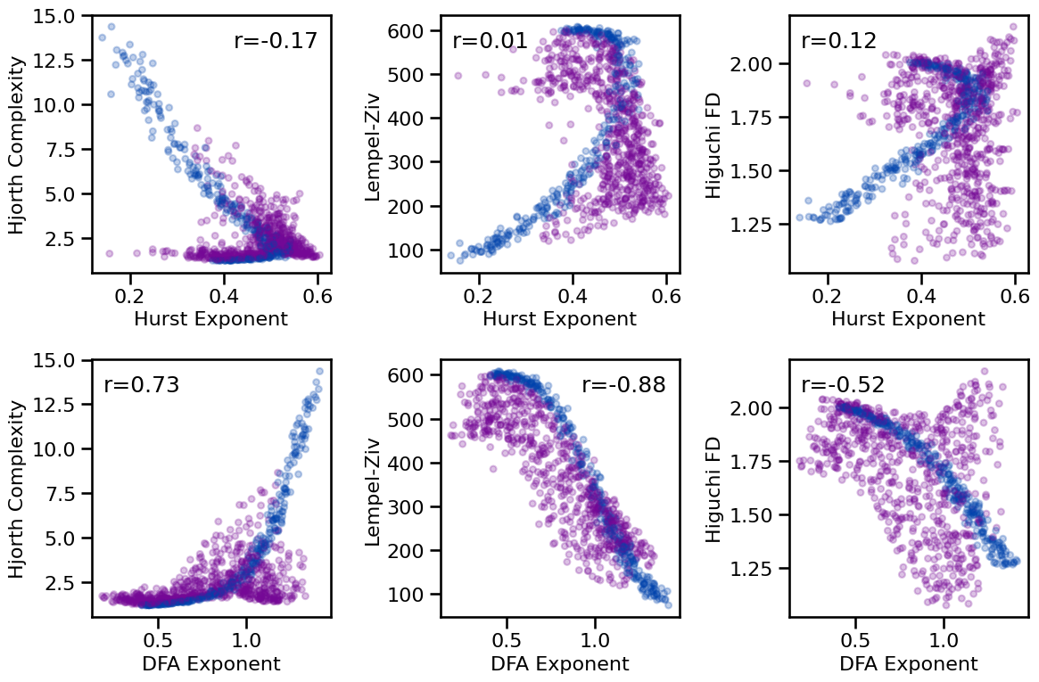
plot_results_rows(results, ['hurst', 'dfa'], ['hjorth_complexity', 'lempelziv', 'higuchi_fd'],
                  tposition=tpos, **dot_kwargs, **fsaver('fluc_compl_comp'))

../_images/42-BetweenComparisons_29_0.png

# Check correlations between fluctuations and complexity measures
print_all_corrs(all_corrs, ['hurst', 'dfa'],
                ['hjorth_complexity', 'lempelziv', 'higuchi_fd'])

Correlations:
  HE     & HJC   :   r=-0.166  CI[-0.237, -0.097],  p=0.000
  HE     & LZC   :   r=+0.005  CI[-0.069, +0.077],  p=0.873
  HE     & HFD   :   r=+0.121  CI[+0.051, +0.190],  p=0.000
  DFA    & HJC   :   r=+0.728  CI[+0.690, +0.761],  p=0.000
  DFA    & LZC   :   r=-0.880  CI[-0.891, -0.866],  p=0.000
  DFA    & HFD   :   r=-0.523  CI[-0.574, -0.470],  p=0.000

Fluctuations to Entropy¶

# Plot comparisons between fluctuation and entropy measures
tpos = np.array([['tl', 'bl'], ['br', 'br']])
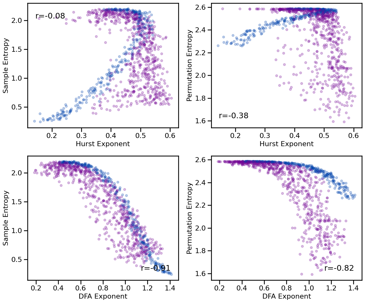
plot_results_rows(results, ['hurst', 'dfa'], ['sample_entropy', 'perm_entropy'],
                  tposition=tpos, **dot_kwargs, figsize=(12, 10), **fsaver('info_fluc_comp'))

../_images/42-BetweenComparisons_32_0.png

# Check correlations between fluctuation and entropy measures
print_all_corrs(all_corrs, ['hurst', 'dfa'],
                ['sample_entropy', 'perm_entropy'])

Correlations:
  HE     & SampEn:   r=-0.077  CI[-0.152, -0.003],  p=0.015
  HE     & PeEn  :   r=-0.378  CI[-0.435, -0.318],  p=0.000
  DFA    & SampEn:   r=-0.911  CI[-0.919, -0.901],  p=0.000
  DFA    & PeEn  :   r=-0.819  CI[-0.833, -0.802],  p=0.000

Complexity to Entropy¶

# Plot comparisons between complexity and entropy measures
tpos = np.array([['tr', 'tl', 'tr'], ['tl', 'tl', 'tr']])
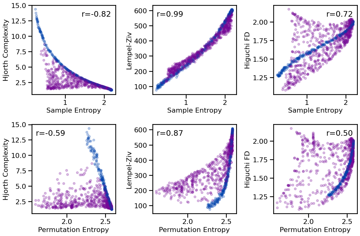
plot_results_rows(results, ['sample_entropy', 'perm_entropy'],
                  ['hjorth_complexity', 'lempelziv', 'higuchi_fd'],
                  tposition=tpos, **dot_kwargs, **fsaver('compl_info_comp'))

../_images/42-BetweenComparisons_35_0.png

# Check correlations between entropy and complexity measures
print_all_corrs(all_corrs, ['sample_entropy', 'perm_entropy'],
                ['hjorth_complexity', 'lempelziv', 'higuchi_fd'])

Correlations:
  SampEn & HJC   :   r=-0.820  CI[-0.854, -0.783],  p=0.000
  SampEn & LZC   :   r=+0.986  CI[+0.982, +0.988],  p=0.000
  SampEn & HFD   :   r=+0.723  CI[+0.677, +0.767],  p=0.000
  PeEn   & HJC   :   r=-0.589  CI[-0.636, -0.539],  p=0.000
  PeEn   & LZC   :   r=+0.870  CI[+0.851, +0.886],  p=0.000
  PeEn   & HFD   :   r=+0.504  CI[+0.443, +0.563],  p=0.000

Time Series - All¶

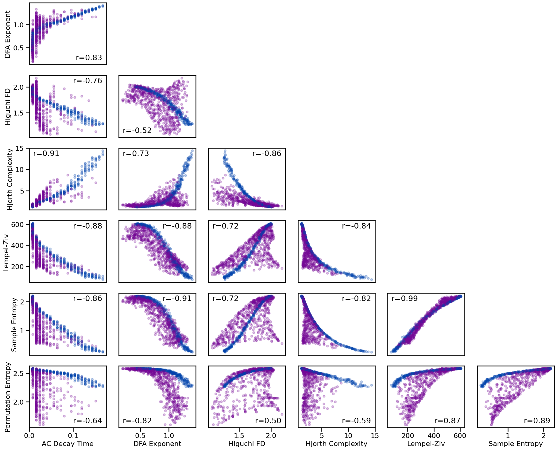
Compare time series methods to each other.

# Define set of measures to plot in group plot
measures = ['autocorr_decay_time', 'dfa', 'higuchi_fd', 'hjorth_complexity',
            'lempelziv', 'sample_entropy', 'perm_entropy']

# Define text positions for the results panels
tpos = np.array([['br', None, None, None, None, None],
                 ['tr', 'bl', None, None, None, None],
                 ['tl', 'tl', 'tr', None, None, None],
                 ['tr', 'tr', 'tl', 'tr', None, None],
                 ['tr', 'tr', 'tl', 'tr', 'tl', None],
                 ['br', 'bl', 'br', 'br', 'br', 'br']])

# Plot results across all measures
plot_results_all(results, measures, **dot_kwargs, wspace=0.01, hspace=0.01,
                 tposition=tpos, figsize=[18.5, 15], **fsaver('all_comp'))

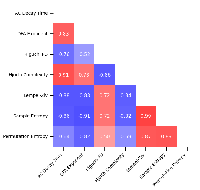
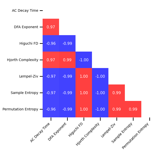
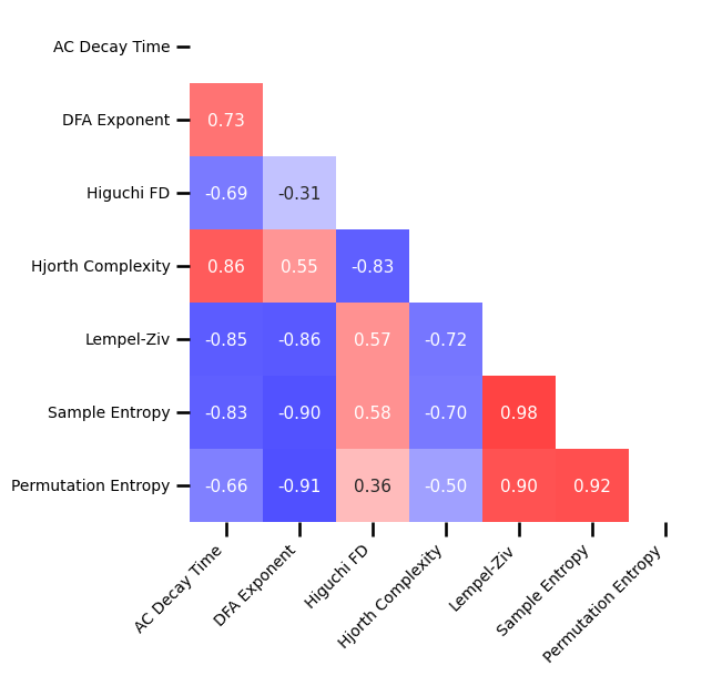
../_images/42-BetweenComparisons_40_0.png

Correlation Matrices¶

# Plot the correlations matrix across all time series measures
plot_corr_matrix(unpack_corrs(all_corrs_ts), cbar=False, figsize=(6, 6), alpha=0.75,
                 xticklabels=ts_labels, yticklabels=ts_labels, **fsaver('corr_mat'))

../_images/42-BetweenComparisons_42_0.png

# Plot the correlations matrix across time series measures for no oscillation
plot_corr_matrix(unpack_corrs(all_corrs_ts_no_osc), cbar=False, figsize=(6, 6), alpha=0.75,
                 xticklabels=ts_labels, yticklabels=ts_labels, **fsaver('corr_mat_no_osc'))

../_images/42-BetweenComparisons_43_0.png

# Plot the correlations matrix across time series measures with an oscillation
plot_corr_matrix(unpack_corrs(all_corrs_ts_osc), cbar=False, figsize=(6, 6), alpha=0.75,
                 xticklabels=ts_labels, yticklabels=ts_labels, **fsaver('corr_mat_osc'))

../_images/42-BetweenComparisons_44_0.png

Exponent Comparisons¶

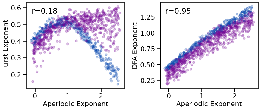
Exponent to Fluctuations¶

# Plot comparisons between exponent and fluctuation measures
plot_results_rows(results, ['specparam'], ['hurst', 'dfa'],
                  **dot_kwargs, tposition='tl', figsize=(9, 4), **fsaver('exp_fluc_comp'))

../_images/42-BetweenComparisons_47_0.png

# Check correlations between exponent and fluctuation measures
print_all_corrs(all_corrs, ['specparam'], ['hurst', 'dfa'])

Correlations:
  Exp(SP) & HE    :   r=+0.182  CI[+0.109, +0.256],  p=0.000
  Exp(SP) & DFA   :   r=+0.949  CI[+0.941, +0.954],  p=0.000

Exponent to Complexity¶

# Plot comparisons between exponent and fluctuation measures
tpos = np.array([['tl', 'tr', 'tl']])
plot_results_rows(results, ['specparam'], ['hjorth_complexity', 'lempelziv', 'higuchi_fd'],
                  tposition=tpos, **dot_kwargs, figsize=(12, 4), **fsaver('exp_compl_comp'))

../_images/42-BetweenComparisons_50_0.png

# Check correlations between exponent and complexity measures
print_all_corrs(all_corrs, ['specparam'], ['hjorth_complexity', 'lempelziv', 'higuchi_fd'])

Correlations:
  Exp(SP) & HJC   :   r=+0.749  CI[+0.706, +0.790],  p=0.000
  Exp(SP) & LZC   :   r=-0.947  CI[-0.953, -0.938],  p=0.000
  Exp(SP) & HFD   :   r=-0.634  CI[-0.686, -0.578],  p=0.000

Exponent to Entropy¶

# Plot comparisons between exponent and entropy measures
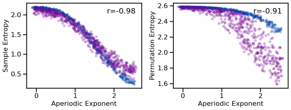
plot_results_rows(results, ['specparam'], ['sample_entropy', 'perm_entropy'],
                  **dot_kwargs, tposition='tr', figsize=(10, 4), **fsaver('exp_info_comp'))

../_images/42-BetweenComparisons_53_0.png

# Check correlations between exponent and entropy measures
print_all_corrs(all_corrs, ['specparam'], ['sample_entropy', 'perm_entropy'])

Correlations:
  Exp(SP) & SampEn:   r=-0.977  CI[-0.980, -0.973],  p=0.000
  Exp(SP) & PeEn  :   r=-0.909  CI[-0.918, -0.899],  p=0.000

Exponent to All¶

# Plot comparison of exponent to all other measures
axes = make_axes(7, 1, figsize=(3.2, 18.5))
tpos = ['tl', 'tl', 'bl', 'tl', 'bl', 'bl', 'bl']
for ind, meas in enumerate(measures):
    plot_dots(results['specparam'], results[meas],
              tposition=tpos[ind], yticks=[],
              xticks=[0.0, 0.5, 1.0, 1.5, 2.0, 2.5] if ind == 6 else [],
              xlabel='Aperiodic Exponent' if ind == 6 else '',
              **dot_kwargs, ax=axes[ind])
plt.gcf().subplots_adjust(hspace=0.18)
if SAVE_FIG: plt.savefig(FIGPATH / ('exp_comp.pdf'))

../_images/42-BetweenComparisons_56_0.png

Correlation Matrices¶

# Extract the correlations between specparam and time domain measures
exp_corrs = np.atleast_2d([all_corrs['specparam'][label][0] for label in ts_measures]).T
exp_corrs_osc = np.atleast_2d([all_corrs_osc['specparam'][label][0] for label in ts_measures]).T
exp_corrs_no_osc = np.atleast_2d([all_corrs_no_osc['specparam'][label][0] for label in ts_measures]).T

# Plot correlations between exponent and time domain measures
plot_corr_matrix(exp_corrs, cbar=False, alpha=0.75,
                 **fsaver('exp_corr_mat'))

../_images/42-BetweenComparisons_59_0.png

# Plot correlations between exponent and time domain measures
plot_corr_matrix(exp_corrs_no_osc, cbar=False, alpha=0.75,
                 **fsaver('exp_corr_mat_no_osc'))

../_images/42-BetweenComparisons_60_0.png

# Plot correlations between exponent and time domain measures
plot_corr_matrix(exp_corrs_osc, cbar=False, alpha=0.75,
                 **fsaver('exp_corr_mat_osc'))

../_images/42-BetweenComparisons_61_0.png

Peak Power Correlations¶

# Plot relationship between specparam exponent and peak power
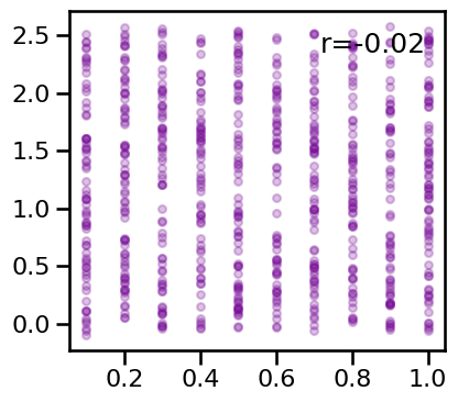
plot_dots(osc_powers, results['specparam'][osc_mask], **dot_kwargs_comb, figsize=(4.5, 4))

../_images/42-BetweenComparisons_63_0.png

# Plot comparison of peak power to all other measures
axes = make_axes(7, 1, figsize=(3, 18), hspace=0.35)
tpos = ['tr', 'tr', 'tl', 'tr', 'tr', 'br', 'bl']
for ind, meas in enumerate(measures):
    plot_dots(osc_powers, results[meas][osc_mask],
              tposition=tpos[ind], yticks=[], xlim=[0, 1.1],
              xticks=[0.0, 0.5, 1.0] if ind == 6 else [],
              xlabel='Oscillatio Power' if ind == 6 else '',
              **dot_kwargs_comb, ax=axes[ind])
if SAVE_FIG: plt.savefig(FIGPATH / ('peak_comp.pdf'))

../_images/42-BetweenComparisons_64_0.png

# Organize correlation values for plotting peak correlation matrix
peak_corrs_mat = np.atleast_2d([peak_corrs[label][0] for label in ts_measures]).T

# Plot correlations between exponent and time domain measures
plot_corr_matrix(peak_corrs_mat, cbar=False, **fsaver('peak_corr_mat'))

../_images/42-BetweenComparisons_66_0.png

Conclusions¶

Comparing between time domain methods, overall we can see that:

Fluctuation and complexity measures have varying, and generally non-linear, relationships to each other
There is generally (though not exclusively) a positive correlation between entropy measures and complexity measures
Entropy is generally negatively correlated to fluctuation measures, though the pattern is non-linear

Comparing time domain methods to exponent, overall we can see that:

Hurst and DFA exponent generally increase with increasing aperiodic exponent
Hjorth complexity increases, but lempel-ziv and higuchi fractal dimension decrease, with increasing exponent
Entropy measures generally decrease with increasing exponent

Aperiodic Methods

Between Method Type Comparisons

Contents

Between Method Type Comparisons¶

Settings¶

Collect Methods¶

Run Simulations¶

Sim Param¶

Correlations¶

Organize Outputs¶

Set up plotting things¶

Fluctuations to Complexity¶

Fluctuations to Entropy¶

Complexity to Entropy¶

Time Series - All¶

Correlation Matrices¶

Exponent Comparisons¶

Exponent to Fluctuations¶

Exponent to Complexity¶

Exponent to Entropy¶

Exponent to All¶

Correlation Matrices¶

Peak Power Correlations¶

Conclusions¶