Fluctuation Analyses¶

This notebook covers ‘fluctuation’ analyses, which examine patterns of fluctuations in time series.

This notebook covers:

The Hurst Exponent
Detrended Fluctuation Analysis

# Setup notebook state
from nbutils import setup_notebook; setup_notebook()

from neurodsp.sim import sim_powerlaw, sim_synaptic_current, sim_combined
from neurodsp.aperiodic.conversions import convert_exponent_alpha
from neurodsp.utils import set_random_seed

# Import custom project code
from apm.io import APMDB
from apm.run import run_sims, run_sims_load
from apm.methods import hurst, dfa
from apm.methods.settings import HURST_PARAMS, DFA_PARAMS
from apm.plts.sims import plot_ap_sims, plot_pe_sims, plot_sims_two
from apm.plts.settings import COLORS
from apm.plts.utils import figsaver
from apm.sim.examples import get_examples, check_examples
from apm.sim.settings import N_SIMS
from apm.sim.defs import SIM_ITERS

Settings¶

# Get current sampling rate
fs = SIM_ITERS.fs

# Add data specific settings to method settings
HURST_PARAMS['fs'] = fs
DFA_PARAMS['fs'] = fs

# Settings for saving figures
SAVE_FIG = True
FIGPATH = APMDB().figs_path / '22_fluctuations'

# Create helper function to manage figsaver settings
fsaver = figsaver(SAVE_FIG, FIGPATH)

# Set the random seed
set_random_seed(111)

# Define collection of example signals
examples = get_examples()

Hurst Exponent¶

The Hurst exponent is a method for measuring the self-similarity of a signal.

# Check Hurst exponent settings
HURST_PARAMS

{'fs': 250, 'n_scales': 10, 'min_scale': 0.1, 'max_scale': 2.0}

Hurst Exponent on Example Signals¶

Compute the Hurst exponent on some example signals.

# Define expected values for Hurst estimation
hurst_expected = {}
hurst_expected['powerlaw'] = 0.5

# Check the calculated hurst exponent, and the expected value
check_examples(examples, hurst, HURST_PARAMS, 'Hurst exponent', hurst_expected)

Computed Hurst exponent:
  powerlaw       : 	 0.5378 	0.50
  synaptic       : 	 0.5766
  knee           : 	 0.5475
  oscillation    : 	 -0.0033
  burst          : 	 nan
  combined       : 	 0.5027
  comb_burst     : 	 0.5049
  comb_peak      : 	 0.4780

/Users/tom/opt/anaconda3/envs/apm/lib/python3.9/site-packages/neurodsp/aperiodic/dfa.py:138: RuntimeWarning: divide by zero encountered in divide
  rs_win = np.ptp(segments, axis=0) / np.std(split_signal(sig, win_len).T, axis=0)

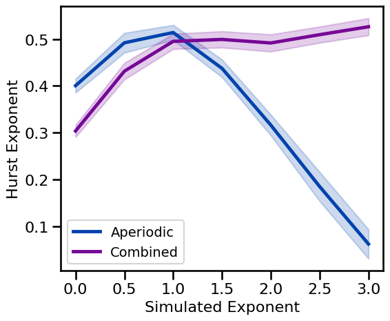
Hurst Exponent: Aperiodic Variations¶

# Run simulations calculating Hurst across exponents
hurst_sims_exp = run_sims(sim_powerlaw, SIM_ITERS['ap_exp'], hurst, HURST_PARAMS, N_SIMS)

# Run simulations calculating Hurst across exponents, with an oscillation
hurst_sims_comb = run_sims(sim_combined, SIM_ITERS['comb_exp'], hurst, HURST_PARAMS, N_SIMS)

# Plot Hurst exponent estimates across aperiodic variations
plot_ap_sims(hurst_sims_exp, hurst_sims_comb, 'Hurst Exponent', **fsaver('hurst_ap'))

Hurst Exponent: Periodic Variations¶

# Run simulations calculating Hurst Exponent across oscillation frequencies
hurst_sims_freq = run_sims(sim_combined, SIM_ITERS['osc_freq'], hurst, HURST_PARAMS, N_SIMS)

# Run simulations calculating Hurst Exponent across oscillation power
hurst_sims_pow = run_sims(sim_combined, SIM_ITERS['osc_pow'], hurst, HURST_PARAMS, N_SIMS)

# Plot Hurst exponent estimates across periodic variations
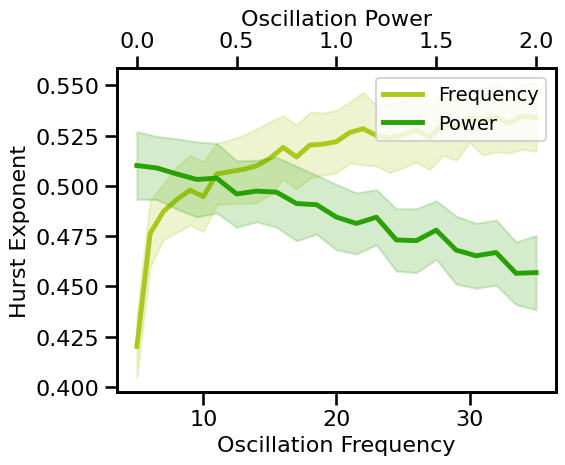
plot_pe_sims(hurst_sims_freq, hurst_sims_pow, 'Hurst Exponent', **fsaver('hurst_pe'))

Hurst Exponent: Knee Variations¶

# Run simulations calculating Hurst Exponent across different timescales
hurst_sims_tscales = run_sims(sim_synaptic_current, SIM_ITERS['syn_tscales'],
                              hurst, HURST_PARAMS, N_SIMS)

# Run simulations calculating Hurst Exponent across different knee parameters (sims from file)
hurst_sims_knee = run_sims_load('ap-knee-' + str(fs), hurst, HURST_PARAMS)

# Plot the estimated hurst exponent across different timescales & knees
plot_sims_two(SIM_ITERS['syn_tscales'].values, hurst_sims_tscales, 'Timescale',
              SIM_ITERS['kn_knee'].values, hurst_sims_knee, 'Knee Parameter',
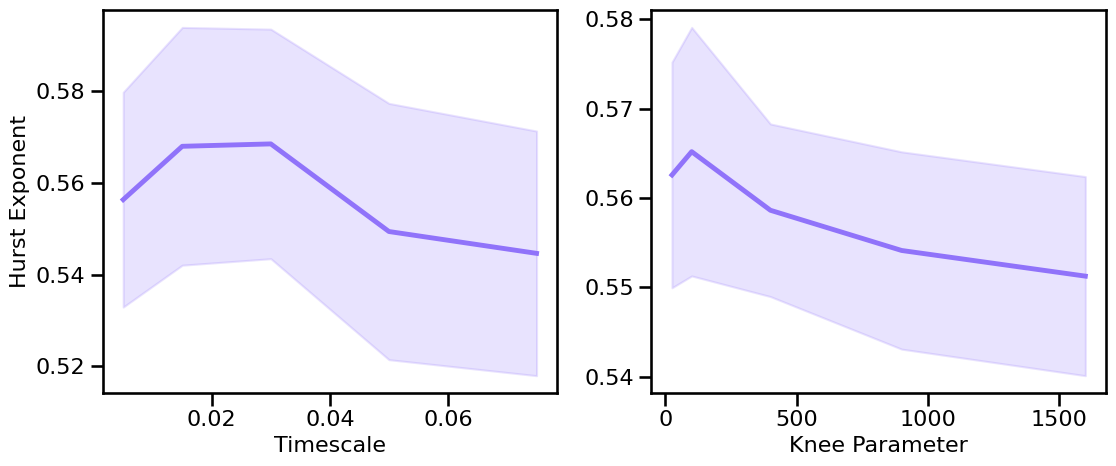
              ylabel='Hurst Exponent', color=COLORS['KN'], **fsaver('hurst_kn_vars'))

Hurst Exponent: Periodic Variations¶

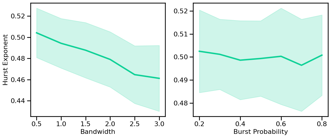
Variations: oscillations bandwidth & burst probability.

# Run simulations calculating Hurst Exponent across peak bandwidth (sims from file)
hurst_sims_bw = run_sims_load('comb-bw-' + str(fs), hurst, HURST_PARAMS)

# Run simulations calculating Hurst Exponent across burst probabilities
hurst_sims_burst = run_sims(sim_combined, SIM_ITERS['comb_burst'],
                            hurst, HURST_PARAMS, N_SIMS)

# Plot the estimated hurst exponent across periodic variations
plot_sims_two(SIM_ITERS['peak_bw'].values, hurst_sims_bw, 'Bandwidth',
              SIM_ITERS['comb_burst'].values, hurst_sims_burst, 'Burst Probability',
              ylabel='Hurst Exponent', color=COLORS['BW'], **fsaver('hurst_pe_vars'))

Detrended Fluctuation Analysis¶

Detrended Fluctuation Analysis is a method for measuring the self-similarity of a signal, and can be applied to measure properties of 1/f-distributed signals.

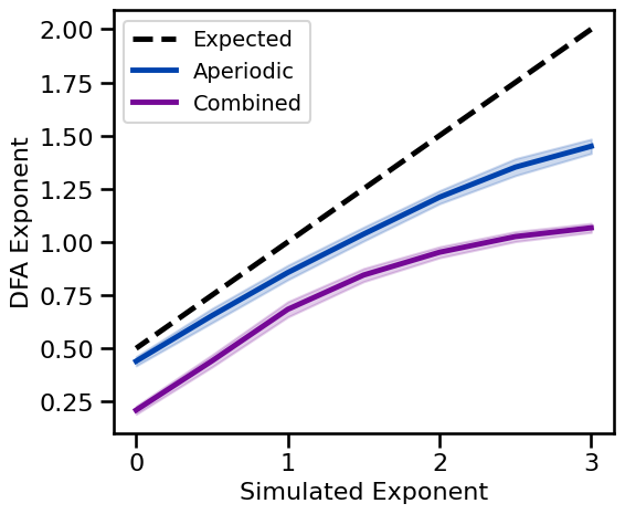
DFA measures an output value, \(\alpha\) which can be interpreted as:

\(\alpha\) < 0.5 anti-correlated signal
\(\alpha\) ~= 0.5: uncorrelated / white noise
\(\alpha\) > 0.5: correlated
- For example: pink noise (\(1/f^1\)) ~= 1 & brown noise (\(1/f^2\)) ~= 1.5

The DFA measure \(\alpha\), should relate to the power spectrum exponent \(f^\chi\) as:

\(\chi\) = 2\(\alpha\) - 1 or
\(\alpha\) = (\(\chi\) + 1) / 2

Settings¶

# Check DFA settings
DFA_PARAMS

{'fs': 250, 'n_scales': 10, 'min_scale': 0.1, 'max_scale': 2.0, 'deg': 1}

DFA on Example Signals¶

# Define expected values for DFA exponent estimation
dfa_expected = {}
dfa_expected['powerlaw'] = convert_exponent_alpha(SIM_ITERS.params['ap']['exponent'])

# Check the computed DFA exponents on some example signals
check_examples(examples, dfa, DFA_PARAMS, 'DFA exponent', dfa_expected)

Computed DFA exponent:
  powerlaw       : 	 0.8164 	1.00
  synaptic       : 	 0.6384
  knee           : 	 0.6589
  oscillation    : 	 0.0078
  burst          : 	 0.0953
  combined       : 	 0.6173
  comb_burst     : 	 0.7456
  comb_peak      : 	 0.6221

DFA Simulations: Aperiodic Variations¶

# Calculate the expected DFA exponent value for each powerlaw exponent
expected_dfa = [convert_exponent_alpha(exp) for exp in SIM_ITERS._iters['ap_exp']['values']]

# Run simulations calculating DFA across exponents
dfa_sims_exp = run_sims(sim_powerlaw, SIM_ITERS['ap_exp'], dfa, DFA_PARAMS, N_SIMS)

# Run simulations calculating DFA across exponents, with an oscillation
dfa_sims_comb = run_sims(sim_combined, SIM_ITERS['comb_exp'], dfa, DFA_PARAMS, N_SIMS)

Plot Aperiodic & Combined Together¶

# Plot DFA measures across exponents
plot_ap_sims(dfa_sims_exp, dfa_sims_comb, 'DFA Exponent',
             expected=expected_dfa, **fsaver('dfa_ap'))

DFA Simulations: Periodic Variations¶

# Run simulations calculating DFA across oscillation frequencies
dfa_sims_freq = run_sims(sim_combined, SIM_ITERS['osc_freq'], dfa, DFA_PARAMS, N_SIMS)

# Run simulations calculating DFA across oscillation power
dfa_sims_pow = run_sims(sim_combined, SIM_ITERS['osc_pow'], dfa, DFA_PARAMS, N_SIMS)

# Plot effect of oscillation variation on DFA exponent
plot_pe_sims(dfa_sims_freq, dfa_sims_pow, 'DFA Exponent', **fsaver('dfa_pe'))

DFA Simulations: Knee Variations¶

# Run simulations calculating DFA Exponent across different timescales
dfa_sims_tscales = run_sims(sim_synaptic_current, SIM_ITERS['syn_tscales'], dfa, DFA_PARAMS, N_SIMS)

# Run simulations calculating DFA Exponent across different knee parameters (sims from file)
dfa_sims_knee = run_sims_load('ap-knee-' + str(fs), dfa, DFA_PARAMS)

# Plot the estimated DFA Exponent across different timescales & knees
plot_sims_two(SIM_ITERS['syn_tscales'].values, dfa_sims_tscales, 'Timescale',
              SIM_ITERS['kn_knee'].values, dfa_sims_knee, 'Knee Parameter',
              ylabel='DFA Exponent', color=COLORS['KN'], **fsaver('dfa_kn_vars'))

DFA Simulations: Periodic Variations¶

# Run simulations calculating DFA Exponent across peak bandwidth (sims from file)
dfa_sims_bw = run_sims_load('comb-bw-' + str(fs), dfa, DFA_PARAMS)

# Run simulations calculating DFA Exponent across burst probabilities
dfa_sims_burst = run_sims(sim_combined, SIM_ITERS['comb_burst'], dfa, DFA_PARAMS, N_SIMS)

# Plot the estimated DFA Exponent across periodic variations
plot_sims_two(SIM_ITERS['peak_bw'].values, dfa_sims_bw, 'Bandwidth',
              SIM_ITERS['comb_burst'].values, dfa_sims_burst, 'Burst Probability',
              ylabel='DFA Exponent', color=COLORS['BW'], **fsaver('dfa_pe_vars'))

Conclusions¶

Overall, we can see the following patterns in these simulations:

Hurst Exponent:

has a parabolic relationship with aperiodic exponent, maximal at an exponent of -1
is less affected by oscillation, increasing slightly with increasing frequency or power

Detrended Fluctuation Analysis:

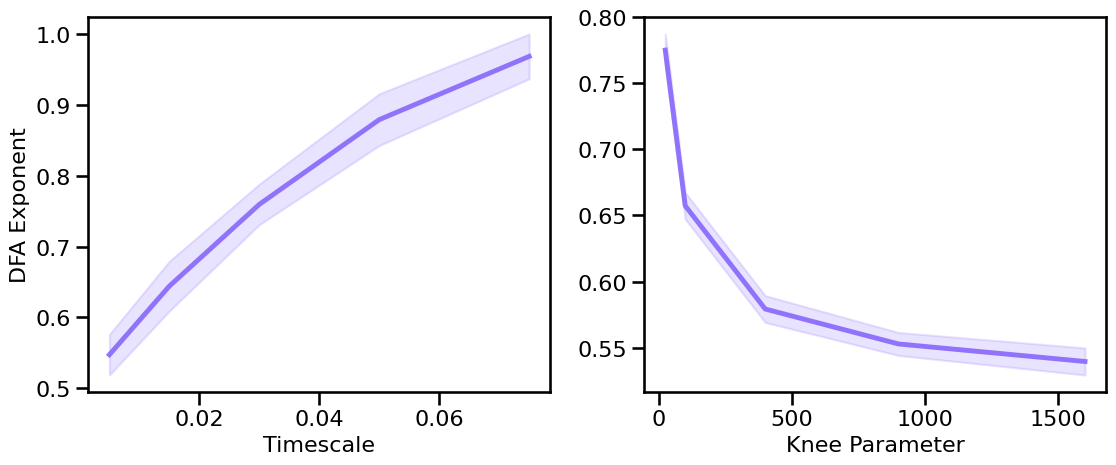
the estimated DFA increases with increasing aperiodic exponent
- the expected DFA results is well estimated across a range \(\chi\) from ~ 0 to 2
- the empirical DFA becomes less close the expected for increasing exponent values
when an oscillation is present, the expected DFA value (for the 1/f) is decreases (is under-estimated)
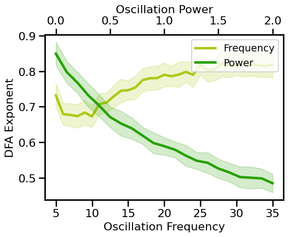
there is a complex relationship between estimated DFA and oscillation frequency
estimated DFA decreases with increasing oscillation power

Aperiodic Methods

Fluctuation Analyses

Contents

Fluctuation Analyses¶

Settings¶

Hurst Exponent¶

Hurst Exponent on Example Signals¶

Hurst Exponent: Aperiodic Variations¶

Hurst Exponent: Periodic Variations¶

Hurst Exponent: Knee Variations¶

Hurst Exponent: Periodic Variations¶

Detrended Fluctuation Analysis¶

Settings¶

DFA on Example Signals¶

DFA Simulations: Aperiodic Variations¶

Plot Aperiodic & Combined Together¶

DFA Simulations: Periodic Variations¶

DFA Simulations: Knee Variations¶

DFA Simulations: Periodic Variations¶

Conclusions¶