Simulation Tests
Contents
Simulation Tests
This notebook introduces how this project examines and evaluates the aperiodic methods using simulations.
Overview
In the simulation method tests, each method is examined independently, and applied to simulated data, to evaluate it’s performance across plausible parameter variations.
Where possible, simulation testing includes estimating the accuracy of each method. For example, the accuracy of methods that estimate 1/f exponents can be evaluated on data simulated to have particular characteristics, and the same can be done for measures that have analytical solutions for expected values on certain kinds of data. In other cases, the analytically expected results are unknown, in which case the simulations are used to characterize how the measures relate to variations across parameters of the simulated data.
Simulations
We use simulated data that systematically varies across parameters of interest to characterize the methods.
Aperiodic Variations
Calculate measures on simulated signals, across variations of aperiodic parameters.
Parameter sweeps include:
variation of aperiodic exponent of powerlaw signals
variation of aperiodic exponent of powerlaw signals with an oscillation present
Periodic Variations
Calculate measures on simulated combined signals, with an oscillation and powerlaw components, across variations of oscillatory parameters.
Parameter sweeps include:
variation of oscillation frequency
variation of oscillation power
Code Approach
Here, we will briefly introduce the general strategy and code used to run the simulations.
run_sims
The overarching function used to run simulations in this section is run_sims.
This approach allows for:
defining a procedure to simulate time series
defining a measure of interest to apply to the simulated time series
applying this measure across simulated instances, sweeping across parameter ranges
# Setup notebook state
from nbutils import setup_notebook; setup_notebook()
import numpy as np
from neurodsp.sim import sim_powerlaw
from neurodsp.sim.io import load_sims
from neurodsp.plts.time_series import plot_multi_time_series
from neurodsp.utils import set_random_seed
# Import custom project code
from apm.io import APMDB
from apm.run import run_sims
from apm.plts import plot_lines
from apm.plts.utils import figsaver
from apm.sim.defs import SIM_ITERS
Settings
# Settings for saving figures
SAVE_FIG = True
FIGPATH = APMDB().figs_path / '13_sim_tests'

# Create helper function to manage figsaver settings
fsaver = figsaver(SAVE_FIG, FIGPATH)
# Settings for loading simulations
SIMPATH = APMDB().sims_path / 'time_series'
# Set the random seed
set_random_seed(111)
Running simulation tests with run_sims
# Check the documentation for `run_sims`
print(run_sims.__doc__)
Compute a measure of interest across a set of simulations.

    Parameters
    ----------
    sim_func : callable
        A function to create the simulations from.
    sim_params : iterable or list of dict
        Simulation parameters for `sim_func`.
    measure_func : callable
        A measure function to apply to the simulated data.
    measure_params : dict
        Input arguments for `measure_func`.
    n_sims : int
        The number of iterations to simulate and calculate measures, per value.
    return_params : bool, default: False
        Whether to collect and return the parameters for the generated simulations.
    outsize : int, optional, default: 1
        Expected size of the measure results.
    warnings_action : {'ignore', 'error', 'always', 'default', 'module, 'once'}
        Filter action for warnings.

    Returns
    -------
    measures : 1d array
        The results of the measures applied to the set of simulations.
Next, we can run an example of using run_sims.
To do so, we will define an example analysis to apply a measure of interest (here, variance) across some simulations of 1/f (powerlaw) data.
# Define settings for simulation
n_sims = 2
# Check the default set of values for the simulation
SIM_ITERS.params['ap']
{'n_seconds': 30, 'fs': 250, 'exponent': -1, 'f_range': (0.5, None)}
# Check the set of values to iterate across
print(SIM_ITERS['ap_exp'].update, ': \t', SIM_ITERS['ap_exp'].values)
exponent : [-3. -2.5 -2. -1.5 -1. -0.5 0. ]
# Run simulations across different aperiodic exponents
results = run_sims(sim_powerlaw, SIM_ITERS['ap_exp'], np.mean, {}, n_sims)
Evaluating Results
After computing the measures, we can examine the results, across different simulation parameters.
Where possible, we also evaluate the accuracy of the computed measures given the expected answer based on the simulated parameters.
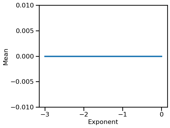
# Plot the computed measures across the different simulation parameters
plot_lines(SIM_ITERS['ap_exp'].values, np.mean(results, 1), np.std(results, 1),
           ylim=[-0.01, 0.01], xlabel='Exponent', ylabel='Mean')

Note that in our example case, computing the signal mean, the simulated signals are normalized such that they all have a mean of 0.
Check Precomputed Simulations
# Set which sims file to load
sims_file_label = 'ap-exp-' + str(SIM_ITERS.fs)
# Load simulations from file
data = load_sims(sims_file_label, SIMPATH)
# Check which feature was updated and set of values
print(data.update, ':', data.values)
exponent : [-3.0, -2.5, -2.0, -1.5, -1.0, -0.5, 0.0]
# # Get the condition labels
# labels = list(data.keys())
# Plot example segments from the first condition
plot_multi_time_series(None, data[0].signals[0:5, 0:5000], **fsaver('time_series1'))

# Plot example segments from the last condition
plot_multi_time_series(None, data[-1].signals[0:5, 0:5000], **fsaver('time_series2'))
