Method Comparisons
Contents
Method Comparisons
This section directly compares between the different methods, using simulated data.
Overview
A key question for interpreting prior work is to consider how the different employed methods relate to each other. To investigate this, this section simulates datasets, and applies different methods to compare their results.
In this section, the main question is the evaluate the relationship between different methods across parameters variations, to evaluate which methods are highly correlated (seeming to refelct the same thing), and which appear to provide independent estimations of the data.
Note that due to large number of possible comparisons across different methods and different simulated parameters, in this section we necessarily restrict the comparison to a selected subset of methods, that are compared pairwise.
Contents
Comparisons between methods are organized into the following groups:
21-ExponentComparisons: comparing methods that directly estimate the aperiodic exponentComparisons between: specparam & IRASA
22-TimeDomainComparisons: comparing time domain methods to each otherComparisons between: fluctuation, complexity, and information measures
23-ExponentvsTimeDomain: comparing exponent and time domain methodsComparisons between: specparam and fluctuation, complexity, and information measures
Simulations
In this section, we will use simulated data to compare methods.
Combined signals
Calculate measures on simulated signals, across variations of aperiodic parameters in combined signals.
Code Approach
Here, we will briefly introduce the general strategy and code used to run the simulations.
run_comparisons
The overarching function used to run simulation comparisons is the run_comparisons function.
This approach allows for:
defining a procedure to simulate time series
defining a set of measures to apply to the simulated time series
applying the set of measures across simulated instances, sampling from parameter ranges
# Import the `run_comparisons` function from the custom code folder
import sys; from pathlib import Path
sys.path.append(str(Path('..').resolve()))
from apm.run import run_comparisons
# Check the documentation for `run_comparisons`
print(run_comparisons.__doc__)
Compute multiple measures of interest across the same set of simulations.

    Parameters
    ----------
    sim_func : callable
        A function to create simulated time series.
    sim_params : dict
        Input arguments for `sim_func`.
    measures : dict
        A measure function to apply to the simulated data.
        The keys should be functions to apply to the data.
        The values should be a dictionary of parameters to use for the method.
    samplers : dict
        Information for how to sample across parameters for the simulations.
        The keys should be string labels of which parameter to update.
        The values should be data ranges to sample for that parameter.
    n_sims : int
        The number of simulations to run.
    verbose : bool, optional, default: False
        Whether to print out simulation parameters.
        Used for checking simulations / debugging.

    Returns
    -------
    outs : dict
        Computed results for each measure across the set of simulated data.
Next, we can run an example of using run_comparisons.
To do so, we will define an example analysis to apply some measures of interest (here, computing the mean and the variance) across samples of simulations of powerlaw data.
import numpy as np
from neurodsp.sim import sim_powerlaw

from apm.sim.settings import SIM_PARAMS_AP
from apm.utils import sampler
# Define the measures to apply to the simulated signals
measures = {np.var : {}, np.mean : {}}

# Define how to sample across parameters, and what ranges to use
samplers = {'update_exp' : sampler(np.arange(-2.5, 0, 0.1))}
# Run comparisons across samples of aperiodic noise
outs = run_comparisons(sim_powerlaw, SIM_PARAMS_AP, measures,
                       samplers, n_sims=5, verbose=True)
{'n_seconds': 30, 'fs': 1000, 'f_range': (0.5, None), 'exponent': -0.19999999999999796}
{'n_seconds': 30, 'fs': 1000, 'f_range': (0.5, None), 'exponent': -0.6999999999999984}
{'n_seconds': 30, 'fs': 1000, 'f_range': (0.5, None), 'exponent': -0.8999999999999986}
{'n_seconds': 30, 'fs': 1000, 'f_range': (0.5, None), 'exponent': -1.5999999999999992}
{'n_seconds': 30, 'fs': 1000, 'f_range': (0.5, None), 'exponent': -1.299999999999999}
# Check output values of computed measures
outs
{'var': array([1., 1., 1., 1., 1.]),
 'mean': array([ 2.46321482e-17,  1.89478063e-17, -9.47390314e-18, -3.03164901e-17,
        -2.98427949e-17])}
Evaluating Results
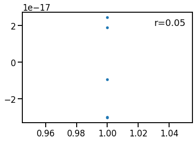
After computing the measures, we can examine the results, comparing between different measurements.
# Import a plot function to visualize the computed measures
from apm.plts import plot_dots
# Plot the computed measures against each other
plot_dots(outs['var'], outs['mean'])
