Simulations
Contents
Simulations
This notebook introduces the simulations used in this project.
%matplotlib inline

import numpy as np
import matplotlib.pyplot as plt

from fooof.sim import gen_power_spectrum

from neurodsp.sim import sim_powerlaw, sim_oscillation, sim_synaptic_current, sim_combined
from neurodsp.utils import create_times, set_random_seed
from neurodsp.spectral import compute_spectrum, rotate_powerlaw
from neurodsp.plts import plot_time_series, plot_power_spectra
# Import custom code
import sys; from pathlib import Path
sys.path.append(str(Path('..').resolve()))
from apm.core.db import APMDB
from apm.plts.data import plot_timeseries_and_psd
from apm.plts.psd import custom_psd_style
# Set plot style
import seaborn as sns
sns.set_context('talk')
Settings
First, we will define some settings for the simulations.
# Set random seed
set_random_seed(111)
# General simulation Settings
n_seconds = 10
fs = 500

# Component parameters
default_exp = -1.0
default_freq = 10
f_range = (1, None)
# Collect together parameters for combined signals
comps_osc = {'sim_powerlaw' : {'exponent' : default_exp},
             'sim_oscillation' : {'freq' : default_freq}}
comps_burst = {'sim_powerlaw' : {'exponent' : default_exp},
               'sim_bursty_oscillation' : {'freq' : default_freq}}
# Create a times vector for time series
times = create_times(n_seconds, fs)
# Plot settings
labels = {'xlabel' : '', 'ylabel' : ''}
tskwargs = {**labels, 'xlim' : [0, times[-1]]}
# Settings for saving figures
SAVE_FIG = True
EXT = '.pdf'
FP = APMDB().figs_path + '/sims/'
Time Series Simulations
Time series are simulated using NeuroDSP.
Powerlaw Signal
First, we can simulate a ‘powerlaw’ signal, a 1/f signal that follow a powerlaw in the frequency domain.
# Simulate a powerlaw signal
sig_pow = sim_powerlaw(n_seconds, fs, default_exp, f_range=f_range)
plot_timeseries_and_psd(times, sig_pow, fs)

Continuous Oscillation
Next, we can simulate an oscillation, in this case, a continuous sinusoid.
# Simulate an oscillation
sig_osc = sim_oscillation(n_seconds, fs, freq=default_freq)
plot_timeseries_and_psd(times, sig_osc, fs)

Combined Signal
Now we can can combine the aperiodic and periodic components from above, and create a combined signal.
# Simulate a combined signal, with an aperiodic and a periodic component
sig_comb = sim_combined(n_seconds, fs, comps_osc)
plot_timeseries_and_psd(times, sig_comb, fs)

Synpatic Signal: Aperiodic Activity with a Knee
There are different possible ways to simulate aperiodic activity.
In this next simulation, we will simulate a ‘synpatic current’ model, which creates aperiodic activity with a knee.
# Simulate aperiodic activity from a synaptic current model
sig_kn = sim_synaptic_current(n_seconds, fs)
plot_timeseries_and_psd(times, sig_kn, fs)

Bursty Oscillation
Oscillations are also not necessarily continuous. We we will simulate a combined signal with a bursty oscillation.
# Simulate a combined signal with a bursty oscillation
sig_burst = sim_combined(n_seconds, fs, comps_burst)
plot_timeseries_and_psd(times, sig_burst, fs)

Example Time Series
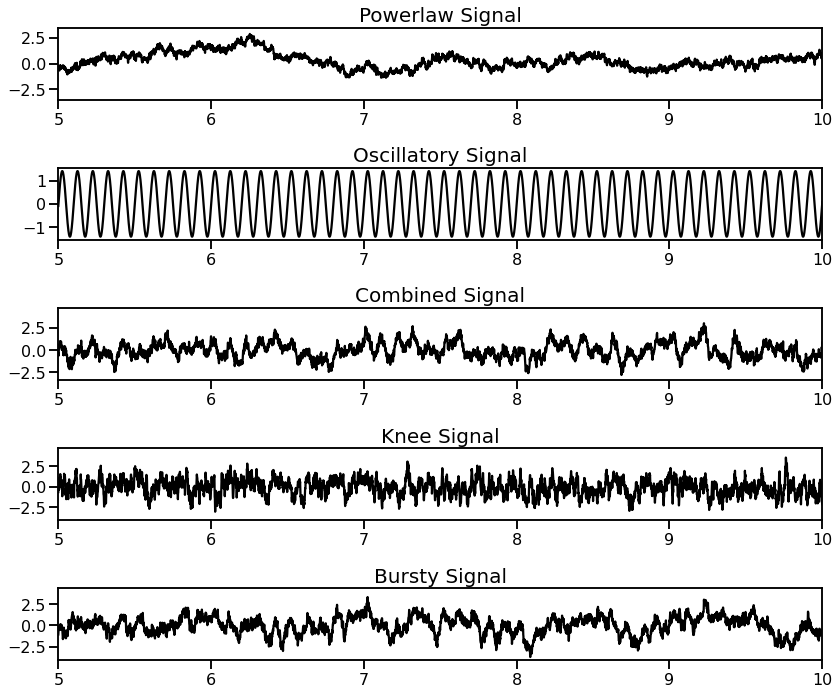
In the notebooks that follow, you will see that measures are applied to a set of ‘example’ time series.
These examples are time series that have been pre-computed, using the functions above.
This set of example signals is shown here.
# Import the pre-computed example signals
from apm.sim.examples import TIMES, SIG_AP, SIG_KN, SIG_OSC, SIG_COMB, SIG_BURST
_, axes = plt.subplots(5, 1, figsize=(12, 10))
plt_kwargs = {'xlabel' : '', 'ylabel' : '', 'xlim' : [5, 10]}
plot_time_series(TIMES, SIG_AP, title='Powerlaw Signal', **plt_kwargs, ax=axes[0])
plot_time_series(TIMES, SIG_OSC, title='Oscillatory Signal', **plt_kwargs, ax=axes[1])
plot_time_series(TIMES, SIG_COMB, title='Combined Signal', **plt_kwargs, ax=axes[2])
plot_time_series(TIMES, SIG_KN, title='Knee Signal', **plt_kwargs, ax=axes[3])
plot_time_series(TIMES, SIG_BURST, title='Bursty Signal', **plt_kwargs, ax=axes[4])
Power Spectrum Simulations
Power spectra are simulated using SpecParam.
Single Peak & Fixed Mode
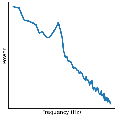
First, we can simulate a power spectrum with a single peak with a 1/f aperiodic component.
freqs, powers = gen_power_spectrum([3, 40], [1, 1], [10, 0.3, 1], nlv=0.025)
plot_power_spectra(freqs, powers, lw=5, ylabel='Power', custom_styler=custom_psd_style,
                   save_fig=SAVE_FIG, file_name='psd_fixed' + EXT, file_path=FP)
Multi-Peak & Knee Mode
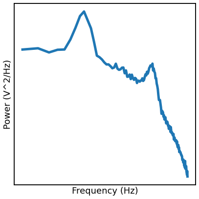
Next, we can simulate a pwoer spectrum that has multiple peaks, and an aperiodic component with a knee.
freqs, powers = gen_power_spectrum([1, 75], [0, 400, 1], [[5, 0.025, 1], [30, 0.02, 4]], nlv=0.001)
plot_power_spectra(freqs, powers, lw=5, custom_styler=custom_psd_style,
                   save_fig=SAVE_FIG, file_name='psd_knee' + EXT, file_path=FP)
Simulating Power Law Signals through Spectral Rotation
The aperiodic components of the above time series simulations are created by spectrally rotating white noise.
This section demonstrates how those simulations work.
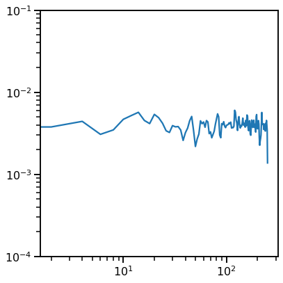
# Simulate a white noise signal
sig = sim_powerlaw(n_seconds, fs, exponent=0)
plot_time_series(times, sig, **tskwargs,
                 save_fig=SAVE_FIG, file_name='rot_ts_pre' + EXT, file_path=FP)

# Compute the power spectrum of the signal
freqs, pows = compute_spectrum(sig, fs, nperseg=250, noverlap=100)
# Plot the power spectrum of the white noise signal
plot_power_spectra(freqs, pows, **labels, ylim=[0.0001, 0.1],
                   save_fig=SAVE_FIG, file_name='rot_psd_pre' + EXT, file_path=FP)
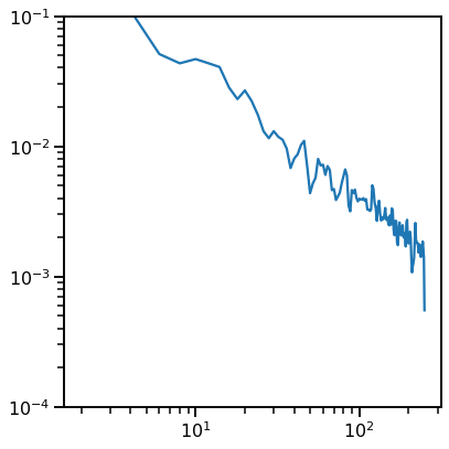
# Rotate the spectrum to desired aperiodic exponent
pows_rot = rotate_powerlaw(freqs, pows, 1, f_rotation=100)
# Plot the power spectrum of the rotated signal
plot_power_spectra(freqs, pows_rot, **labels, ylim=[0.0001, 0.1],
                   save_fig=SAVE_FIG, file_name='rot_psd_post' + EXT, file_path=FP)
# Get the rotated signal, back in the time domain
#   Note: this step directly uses the NDSP function, which rotates a new signal behind the scenes
sig = sim_powerlaw(n_seconds, fs, exponent=-1)
# Plot the time series of the rotated signal, with the desired aperiodic exponent
plot_time_series(times, sig, **tskwargs,
                 save_fig=SAVE_FIG, file_name='rot_ts_post' + EXT, file_path=FP)
