Methods¶

This section introduces and characterizes the methods included in this project.

Overview¶

In this section, each method is examined independently, and applied to simulated data, to evaluate it’s performance across plausible parameter variations.

Where possible, simulation testing includes estimating the accuracy of each method. For example, the accuracy of methods that estimate 1/f exponents can be evaluated on data simulated to have particular characteristics, and the same can be done for measures that have analytical solutions for expected values on certain kinds of data. In other cases, the analytically expected results are unknown, in which case the simulations are used to characterize how the measures relate to variations across parameters of the simulated data.

Contents¶

Methods that are included in this project:

11-SpectralFitting: measuring aperiodic parameters by fitting the power spectrum
- methods: line fitting, robust line fitting, spectral parameterization
12-IRASA: the irregular resampling and auto-spectral analysis algorithm
- methods: IRASA
13-AutoCorrelation: auto-correlation measures
- methods: auto correlation
14-Fluctuations: includes the Hurst exponent and
- methods: Hurst exponent, detrended fluctuation analysis (DFA)
15-Complexity: time series complexity measures, including
- methods: Hjorth parameters, fractal measures: Higuchi, Katz, Petrosian
16-Information: information
- sample entropy, permutation entropy, approximate entropy, spectral entropy

Simulations¶

In this section, we will use simulated data to characterize methods.

Aperiodic Variations¶

Calculate measures on simulated signals, across variations of aperiodic parameters.

Parameter sweeps include:

variation of aperiodic exponent of powerlaw signals
variation of aperiodic exponent of powerlaw signals with an oscillation present

Periodic Variations¶

Calculate measures on simulated combined signals, with an oscillation and powerlaw components, across variations of oscillatory parameters.

Parameter sweeps include:

variation of oscillation frequency
variation of oscillation power

Code Approach¶

Here, we will briefly introduce the general strategy and code used to run the simulations.

run_sims¶

The overarching function used to run simulations in this section is run_sims.

This approach allows for:

defining a procedure to simulate time series
defining a measure of interest to apply to the simulated time series
applying this measure across simulated instances, sweeping across parameter ranges

# Import the `run_sims` function from the custom code folder
import sys; from pathlib import Path
sys.path.append(str(Path('..').resolve()))
from apm.run import run_sims

# Check the documentation for `run_sims`
print(run_sims.__doc__)

Compute a measure of interest across a set of simulations.

    Parameters
    ----------
    sim_func : callable
        A function to create the simulations from.
    sim_params : dict
        Input arguments for `sim_func`.
    measure_func : callable
        A measure function to apply to the simulated data.
    measure_params : dict
        Input arguments for `measure_func`.
    update : {'update_exp', 'update_freq', 'update_pow', 'update_comb_exp'} or callable
        Specifies which parameter to update in simulation parameters.
    values : list or 1d array
        A parameter to step across and re-run measure calculations for.
    n_sims : int, optional, default: 10
        The number of iterations to simulate and calculate measures, per value.
    avg_func : callable, optional, default: np.mean
        The function to calculate the average for a particular parameter value.
    var_func : callable, optional
        The function to calculate the variability for a particular parameter value.
        If None, variability is not computed.

    Returns
    -------
    measures : 1d array
        The results of the measures applied to the set of simulations.

    Notes
    -----
    - For each parameter value, the average measure across `n_sims`
      of simulations is computed and returned.
    

Next, we can run an example of using run_sims.

To do so, we will define an example analysis to apply a measure of interest (here, variance) across some simulations of 1/f (powerlaw) data.

# Import numpy
import numpy as np

# Import simulation function
from neurodsp.sim import sim_powerlaw

# Import default simulation settings
from apm.sim.settings import SIM_PARAMS_AP

# Define settings for simulation
exponents = [1, 1.5, 2]
n_sims = 2

# Check the predefined default settings for the simulation
SIM_PARAMS_AP

{'n_seconds': 30, 'fs': 1000, 'f_range': (0.5, None)}

# Run simulations across different aperiodic exponents
out, var = run_sims(sim_powerlaw, SIM_PARAMS_AP, np.mean, {}, 
                    'update_exp', exponents, n_sims, var_func=np.std)

Evaluating Results¶

After computing the measures, we can examine the results, across different simulation parameters.

Where possible, we also evaluate the accuracy of the computed measures given the expected answer based on the simulated parameters.

# Import a plot function to visualize the computed measures
from apm.plts import plot_lines

# Plot the computed measures across the different simulation parameters
plot_lines(exponents, out, var, ylim=[-0.01, 0.01],
           xlabel='Exponent', ylabel='Mean')

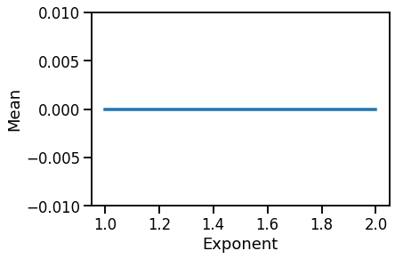
Note that in our example case, computing the signal mean, the simulated signals are normalized such that they all have a mean of 0.

Aperiodic Methods

Methods

Contents