Fluctuation Analyses¶

This notebook covers ‘fluctuation’ analyses, which examine patterns of fluctuations in time series.

This notebook covers:

The Hurst Exponent
Detrended Fluctuation analyses

import numpy as np
import matplotlib.pyplot as plt

from neurodsp.sim import sim_powerlaw, sim_synaptic_current, sim_combined
from neurodsp.aperiodic import compute_fluctuations
from neurodsp.utils import set_random_seed
from neurodsp.aperiodic.conversions import convert_exponent_alpha, convert_alpha_exponent

# Import custom code
import sys; from pathlib import Path
sys.path.append(str(Path('..').resolve()))

from apm.run import run_sims
from apm.methods import hurst, dfa
from apm.methods.settings import HURST_PARAMS, DFA_PARAMS
from apm.plts import plot_lines
from apm.plts.settings import AP_COL, COMB_COL
from apm.sim.settings import FS, SIM_PARAMS_AP, SIM_PARAMS_COMB, EXPS, FREQS, POWERS, N_SIMS, EXP
from apm.sim.examples import SIG_AP, SIG_KN, SIG_OSC, SIG_COMB

Settings¶

# Set the random seed
set_random_seed(111)

# Notebook settings
SAVE_FIG = False

Hurst Exponent¶

The Hurst exponent is a method for measuring the self-similarity of a signal.

# Check Hurst exponent settings
HURST_PARAMS

{'fs': 1000, 'n_scales': 10, 'min_scale': 0.1, 'max_scale': 2.0}

Hurst Exponent on Example Signals¶

Compute the Hurst exponent on some example signals.

# Check the calculated hurst exponent, and the expected value
print('Computed Hurst signals:')
print('  powerlaw: \t {:1.4f} \t {:1.2f}'.format(hurst(SIG_AP, **HURST_PARAMS), 0.5))
print('  osc:      \t {:6.4f}'.format(hurst(SIG_OSC, **HURST_PARAMS)))
print('  combined: \t {:1.4f}'.format(hurst(SIG_COMB, **HURST_PARAMS)))
print('  knee:     \t {:1.4f}'.format(hurst(SIG_KN, **HURST_PARAMS)))

Computed Hurst signals:
  powerlaw: 	 0.6735 	 0.50
  osc:      	 -0.0033
  combined: 	 0.4768
  knee:     	 0.5425

Hurst Exponent: Aperiodic Variations¶

# Run a set of simulations, calculating Hurst across exponents
outs = run_sims(sim_powerlaw, SIM_PARAMS_AP, hurst, HURST_PARAMS,
                'update_exp', EXPS, N_SIMS, var_func=np.std)
hurst_sims_exp, hurst_sims_exp_var = outs

# Plot Hurst measures
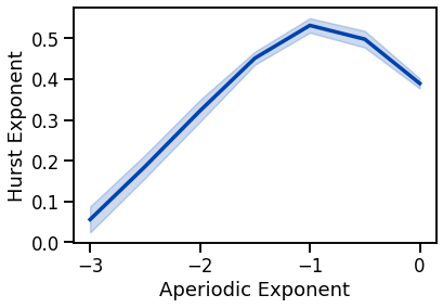
plot_lines(EXPS, hurst_sims_exp, hurst_sims_exp_var, color=AP_COL)
plot_lines(xlabel='Aperiodic Exponent', ylabel='Hurst Exponent')
plot_lines(save_fig=SAVE_FIG, file_name='hurst_exp', file_path='fluctuations')

# Run a set of simulations, calculating Hurst across exponents, with an oscillation
outs = run_sims(sim_combined, SIM_PARAMS_COMB, hurst, HURST_PARAMS,
                'update_comb_exp', EXPS, N_SIMS, var_func=np.std)
hurst_sims_comb, hurst_sims_comb_var = outs

# Plot Hurst measures
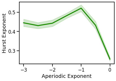
plot_lines(EXPS, hurst_sims_comb, hurst_sims_comb_var, color=COMB_COL)
plot_lines(xlabel='Aperiodic Exponent', ylabel='Hurst Exponent')
plot_lines(save_fig=SAVE_FIG, file_name='hurst_comb', file_path='fluctuations')

Plot Aperiodic & Combined Together¶

# Plot Hurst measures
plot_lines(figsize=(6, 5))
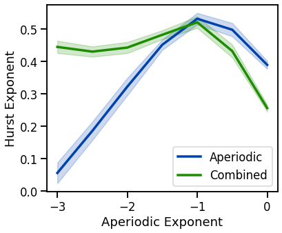
plot_lines(EXPS, hurst_sims_exp, hurst_sims_exp_var, color=AP_COL, label='Aperiodic')
plot_lines(EXPS, hurst_sims_comb, hurst_sims_comb_var, color=COMB_COL, label='Combined')
plot_lines(xlabel='Aperiodic Exponent', ylabel='Hurst Exponent')
plot_lines(save_fig=SAVE_FIG, file_name='hurst_both', file_path='fluctuations')

Hurst Exponent: Periodic Variations¶

# Run a set of simulations, calculating Hurst Exponent across oscillation frequencies
outs = run_sims(sim_combined, SIM_PARAMS_COMB, hurst, HURST_PARAMS,
                'update_freq', FREQS, N_SIMS, var_func=np.std)
hurst_sims_freq, hurst_sims_freq_var = outs

# Run a set of simulations, calculating Hurst across oscillation power
outs = run_sims(sim_combined, SIM_PARAMS_COMB, hurst, HURST_PARAMS,
                'update_pow', POWERS, N_SIMS, var_func=np.std)
hurst_sims_pow, hurst_sims_pow_var = outs

# Plot effect of oscillation variation on Hurst exponent
fig, axes = plt.subplots(1, 2, figsize=(14, 5))
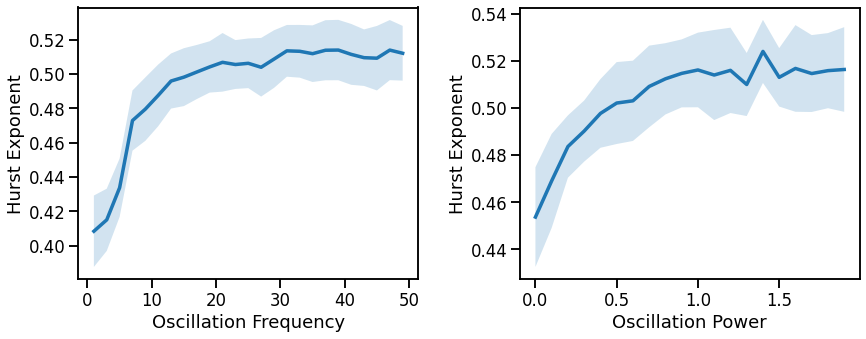
plot_lines(FREQS, hurst_sims_freq, hurst_sims_freq_var, ax=axes[0])
plot_lines(xlabel='Oscillation Frequency', ylabel='Hurst Exponent', ax=axes[0])
plot_lines(POWERS, hurst_sims_pow, hurst_sims_pow_var, ax=axes[1])
plot_lines(xlabel='Oscillation Power', ylabel='Hurst Exponent', ax=axes[1])
plt.subplots_adjust(wspace=0.3)
plot_lines(save_fig=SAVE_FIG, file_name='hurst_osc_both', file_path='fluctuations')

Detrended Fluctuation Analysis¶

Detrended Fluctuation Analysis is a method for measuring the self-similarity of a signal, and can be applied to measure properties of 1/f-distributed signals.

DFA measures an output value, \(\alpha\) which can be interpreted as:

\(\alpha\) < 0.5 anti-correlated signal
\(\alpha\) ~= 0.5: uncorrelated / white noise
\(\alpha\) > 0.5: correlated
- For example: pink noise (\(1/f^1\)) ~= 1 & brown noise (\(1/f^2\)) ~= 1.5

The DFA measure \(\alpha\), should relate to the power spectrum exponent \(f^\chi\) as:

\(\chi\) = 2\(\alpha\) - 1 or
\(\alpha\) = (\(\chi\) + 1) / 2

In this notebook, we will explore:

applying DFA to neural time signals
how DFA measures relate to different properties of neural time series
compare DFA measures to other measures of 1/f.

Notes¶

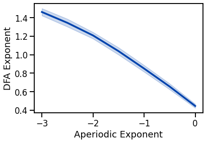
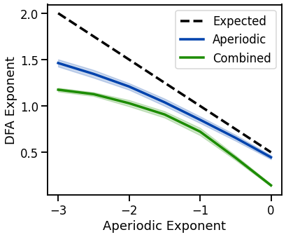
It looks like the expected relationship between DFA & 1/f appears to be true in the range of \(\chi\) from -3 to 0.
- It seems like it breaks down with exponent of less than -3
- It also doesn’t seem to hold for exponents > 0
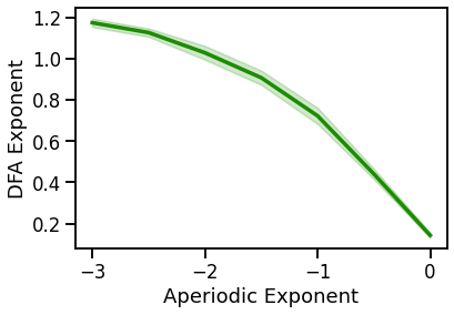
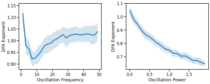
The presence of an oscillations decreases measures DFA
- Increasing the frequency of the oscillation further decreases measured DFA
- Increasing the relative power of the oscillation further decreases measured DFA
It would appear that given a combined signal, the measured DFA is upper-bound at the expected DFA given the exponent

Settings¶

# Check DFA settings
DFA_PARAMS

{'fs': 1000, 'n_scales': 10, 'min_scale': 0.1, 'max_scale': 2.0, 'deg': 1}

DFA on Example Signals¶

# Check the computed DFA exponents on some example signals
print('DFA exponents:')
print('  powerlaw: \t {:1.4f} \t {:1.2f}'.format(dfa(SIG_AP, **DFA_PARAMS),
                                                 convert_exponent_alpha(EXP)))
print('  osc:      \t {:1.4f}'.format(dfa(SIG_OSC, **DFA_PARAMS)))
print('  combined: \t {:1.4f}'.format(dfa(SIG_COMB, **DFA_PARAMS)))
print('  knee:     \t {:1.4f}'.format(dfa(SIG_KN, **DFA_PARAMS)))

DFA exponents:
  powerlaw: 	 1.2865 	 1.25
  osc:      	 0.0078
  combined: 	 0.9248
  knee:     	 0.6050

DFA Simulations: Aperiodic Variations¶

# Calculate the expected DFA exponent value for each powerlaw exponent
expected = [convert_exponent_alpha(exp) for exp in EXPS]

# Run a set of simulations, calculating DFA across exponents
outs = run_sims(sim_powerlaw, SIM_PARAMS_AP, dfa, DFA_PARAMS,
                'update_exp', EXPS, N_SIMS, var_func=np.std)
dfa_sims_exp, dfa_sims_exp_var = outs

# Plot approximate entropy measures across exponent values
plot_lines(EXPS, dfa_sims_exp, dfa_sims_exp_var, color=AP_COL)
plot_lines(xlabel='Aperiodic Exponent', ylabel='DFA Exponent')
plot_lines(save_fig=SAVE_FIG, file_name='dfa_exp', file_path='fluctuations')

# Run a set of simulations, calculating DFA across exponents, with an oscillation
outs = run_sims(sim_combined, SIM_PARAMS_COMB, dfa, DFA_PARAMS,
                'update_comb_exp', EXPS, N_SIMS, var_func=np.std)
dfa_sims_comb, dfa_sims_comb_var = outs

# Plot approximate entropy measures across exponent values
plot_lines(EXPS, dfa_sims_comb, dfa_sims_comb_var, color=COMB_COL)
plot_lines(xlabel='Aperiodic Exponent', ylabel='DFA Exponent')
plot_lines(save_fig=SAVE_FIG, file_name='dfa_comb', file_path='fluctuations')

Plot Aperiodic & Combined Together¶

# Plot DFA measures
plot_lines(figsize=(6, 5))
plot_lines(EXPS, expected, color='k', linestyle='--', label='Expected');
plot_lines(EXPS, dfa_sims_exp, dfa_sims_exp_var, color=AP_COL, label='Aperiodic')
plot_lines(EXPS, dfa_sims_comb, dfa_sims_comb_var, color=COMB_COL, label='Combined')
plot_lines(xlabel='Aperiodic Exponent', ylabel='DFA Exponent')
plot_lines(save_fig=SAVE_FIG, file_name='dfa_both', file_path='fluctuations')

DFA Simulations: Periodic Variations¶

# Run a set of simulations, calculating DFA across oscillation frequencies
outs = run_sims(sim_combined, SIM_PARAMS_COMB, dfa, DFA_PARAMS,
                'update_freq', FREQS, N_SIMS, var_func=np.std)
dfa_sims_freq, dfa_sims_freq_var = outs

# Run a set of simulations, calculating DFA across oscillation power
outs = run_sims(sim_combined, SIM_PARAMS_COMB, dfa, DFA_PARAMS,
                'update_pow', POWERS, N_SIMS, var_func=np.std)
dfa_sims_pow, dfa_sims_pow_var = outs

# Plot effect of oscillation variation on Hurst exponent
fig, axes = plt.subplots(1, 2, figsize=(14, 5))
plot_lines(FREQS, dfa_sims_freq, dfa_sims_freq_var, ax=axes[0])
plot_lines(xlabel='Oscillation Frequency', ylabel='DFA Exponent', ax=axes[0])
plot_lines(POWERS, dfa_sims_pow, dfa_sims_pow_var, ax=axes[1])
plot_lines(xlabel='Oscillation Power', ylabel='DFA Exponent', ax=axes[1])
plt.subplots_adjust(wspace=0.3)
plot_lines(save_fig=SAVE_FIG, file_name='dfa_osc_both', file_path='fluctuations')

Conclusions¶

Overall, we can see the following patterns in these simulations:

Hurst Exponent:

has a parabolic relationship with aperiodic exponent, maximal at an exponent of -1
is less affected by oscillation, increasing slightly with increasing frequency or power

Detrended Fluctuation Analysis:

decreases with decreasing aperiodic exponent
when an oscillation is present, the expected DFA value (for the 1/f) is under-estimated
has a complex relationship with oscillation frequency, decreases with increasing oscillation power

Aperiodic Methods

Fluctuation Analyses

Contents

Fluctuation Analyses¶

Settings¶

Hurst Exponent¶

Hurst Exponent on Example Signals¶

Hurst Exponent: Aperiodic Variations¶

Plot Aperiodic & Combined Together¶

Hurst Exponent: Periodic Variations¶

Detrended Fluctuation Analysis¶

Notes¶

Settings¶

DFA on Example Signals¶

DFA Simulations: Aperiodic Variations¶

Plot Aperiodic & Combined Together¶

DFA Simulations: Periodic Variations¶

Conclusions¶